Guides
Design a variant library
Wild type to ordered library, ranked by a protein language model. The ranking is a screening plan, not an answer — and the outcome log is what makes round two better than round one.
Updated 31 July 2026
All documentation
On this page
This improves an existing protein along an existing axis — stability, expression, mild activity tuning. It is not de novo design, and the distinction matters for what you should expect from the ranking.
Provide a wild type
Accepted: FASTA, SnapGene, GenBank, EMBL, raw DNA, or raw protein. Upload a file or paste text; the cap is 8 MiB.
The engine detects what it received. Two cases need a decision from you:
- A plasmid or multi-CDS record surfaces a CDS picker. The build refuses to
guess which coding sequence you meant — that returns
kind:
  needs_cds_choice
with the options listed. - Raw DNA with multiple stop codons triggers six-frame ORF discovery, and you pick the frame.
Ambiguous bases have to be resolved first
ESM-2 scoring needs a fully determined wild type. N, R, Y and the rest
of the IUPAC ambiguity codes are rejected rather than guessed at.
You can also press Identify via NCBI BLAST to resolve what the protein actually is, which returns UniProt accessions and AlphaFold links for the structure viewer. That step sends your sequence to NCBI.
Set five parameters
| Setting | Default | What raising it does |
|---|---|---|
| Model | ESM-2 35M | 650M and 3B appear marked “Pro · GPU (coming soon)” and are not available |
| Percentile | 85 | Widens the pool of single-site mutations the search draws from |
Variants (k) |
30 | More designs, longer run |
| Max mutations | 5 | Deeper combinations, sharply lower functional retention |
| Host | E. coli | Switches the codon-usage table (also yeast, human) |
Understand what the ranking is
ESM-2 computes ΔLL for every position × 19 substitutions — how much more or less plausible the mutant is than the wild type, given the rest of the sequence. Simulated annealing then searches combinations, using cumulative ΣΔLL as fitness with penalties for stop codons and repeated positions.
Functional retention falls steeply with mutation count:
| Mutations per variant | Approximate functional retention |
|---|---|
| 1–2 | 70–85% |
| 3–4 | 50–70% |
| 5–6 | 30–55% |
| 7–8 | 15–40% |
| 9+ | < 25% |
Cap at 3–4 unless you have a structural reason not to
The model sees evolutionary plausibility learned from roughly 65 million UniRef50 sequences: conservation, coevolution, sequence context. It does not see structure, it does not know which residue is your active site, and it cannot see epistasis between the mutations it just combined. Membrane proteins, intrinsically disordered proteins and multi-domain assemblies are where it is weakest.
Published benchmark figures are on /api/benchmarks — a 2026-07-17 run over
three public deep-mutational-scanning datasets and 7,761 variants gave a median
Spearman correlation of 0.5165 and median top-decile precision of 0.386,
using the 35M model. Those are the only figures that exist; there are none for
the larger models.
Read the library
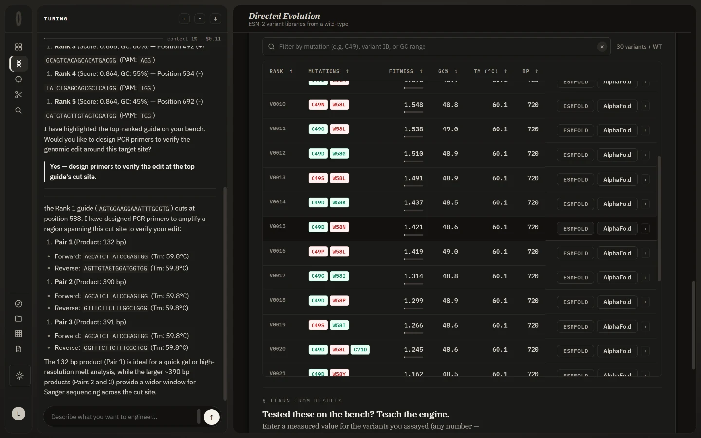
Six columns, with the wild type prepended as a reference row. A real run over the 720 nt EGFP CDS at the defaults:
RANK   MUTATIONS    FITNESS   GC%    TM (°C)   BP
WT     wild type    —         48.9   60.1      720
V0001  C49D,W58L    2.300     48.8   60.1      720
V0002  C49D,W58I    2.076     48.5   60.1      720
…
V0030  C49S,W58F    0.842     48.6   60.1      720
Fitness is the cumulative ΣΔLL described above, so it is comparable within one library and meaningless across two. The wild type has no fitness by definition — it is the baseline everything else is scored against.
Every row carries ESMFold and AlphaFold buttons that open a structure for that specific variant, and an expander for the full DNA and translation.
Your ranking is nudged by other labs’ measurements
The summary line reports the prior it used — in this run, “informed by pooled results from other labs (276 substitution types)”. Where enough labs have logged a measured outcome for a substitution type, that evidence adjusts the zero-shot score. Only aggregate substitution statistics are pooled; individual sequences are not shared.
Filter the table
The results table takes filter expressions directly:
gc>50
tm>58
fitness>2
bp<800
W58L
C49
A bare mutation like W58L matches variants carrying it; C49 matches anything
mutated at position 49. Numeric expressions compare the corresponding column.
Codon optimisation happens automatically
Each variant is reverse-translated against the host’s codon-usage table, then
synonymously scrubbed of BsaI (GGTCTC), BsmBI (CGTCTC) and NotI
(GCGGCCGC) sites — on both strands, because Type IIS enzymes cut either. That
is what lets the insert survive Golden Gate assembly and vendor synthesis
screening.
The export carries forward and reverse primers, their Tm and GC, and a suggested
annealing temperature of min(Tm) − 5 °C. A WT pseudo-row is prepended so you
can order the unmutated reference alongside as a control.
Export
csv, tsv, fasta (protein), fasta-dna, gb, xlsx or json. You can
also edit a single variant’s DNA in place — the engine re-derives the
translation, the mutation diff and the PCR metrics, and rejects an edit that
breaks the frame or introduces a premature stop, because vendors will reject it
too.
Close the loop
Screen the library, then log the outcomes — the measured value for each variant you tested. Round 2 re-ranks using a surrogate model trained on what you actually measured, rather than on the prior alone.
Interaction radar scans for epistasis between positions, which is the thing the zero-shot ranking is structurally blind to. Both are capped at 500 aa of protein.
This is the only step that creates new information
Everything before it is prediction from a model that has never seen your protein. The outcome log is measurement, and it is the reason round two ranks better than round one.